
| 일 | 월 | 화 | 수 | 목 | 금 | 토 |
|---|---|---|---|---|---|---|
| 1 | 2 | 3 | ||||
| 4 | 5 | 6 | 7 | 8 | 9 | 10 |
| 11 | 12 | 13 | 14 | 15 | 16 | 17 |
| 18 | 19 | 20 | 21 | 22 | 23 | 24 |
| 25 | 26 | 27 | 28 | 29 | 30 | 31 |
Tags
- 모두를 위한 머신러닝
- deep learning
- BOJ
- ML
- CSAP
- 정렬
- 한화오션
- sung kim
- SQL
- 큐
- 시간초과
- Machine learning
- deque
- 프로그래머스
- softmax
- stl
- join
- sort
- Neural Network
- PIR
- Linear Regression
- Programmers
- 백준
- mysql
- c++
- 알고리즘 고득점 kit
- DFS
- Queue
- TensorFlow
- 모두를 위한 딥러닝
Archives
- Today
- Total
hello, world!
[ML lab 07-1] training/test dataset, learning rate, normalization 본문
AI/모두를 위한 ML (SungKim)
[ML lab 07-1] training/test dataset, learning rate, normalization
ferozsun 2021. 2. 20. 16:41[내가 만든 모델이 얼마나 훌륭한지 어떻게 평가할까?]
training datasets을 통해 평가하는 것은 좋은 방법이 아니다.
dataset을 training set과 test set으로 나누는 것이 핵심!
training dataset: 모델을 학습시킬 때 사용한다.
test dataset: 학습된 모델의 성능을 계산할 때 사용한다.
import tensorflow.compat.v1 as tf
tf.disable_v2_behavior()

# training data
# 모델을 학습시킬 때만 사용
x_data = [[1, 2, 1], [1, 3, 2], [1, 3, 4], [1, 5, 5], [1, 7, 5], [1, 2, 5], [1, 6, 6], [1, 7, 7]]
y_data = [[0, 0, 1], [0, 0, 1], [0, 0, 1], [0, 1, 0], [0, 1, 0], [0, 1, 0], [1, 0, 0], [1, 0, 0]]

# test data
# Evaluation our model using this test dataset
x_test = [[2, 1, 1], [3, 1, 2], [3, 3, 4]]
y_test = [[0, 0, 1], [0, 0, 1], [0, 0, 1]]


X = tf.placeholder("float", [None, 3])
Y = tf.placeholder("float", [None, 3])
W = tf.Variable(tf.random_normal([3, 3]))
b = tf.Variable(tf.random_normal([3]))

hypothesis = tf.nn.softmax(tf.matmul(X, W) + b)
cost = tf.reduce_mean(-tf.reduce_sum(Y * tf.log(hypothesis), axis = 1))
optimizer = tf.train.GradientDescentOptimizer(learning_rate = 0.1).minimize(cost)

# Correct prediction Test model
prediction = tf.arg_max(hypothesis, 1)
is_correct = tf.equal(prediction, tf.arg_max(Y, 1))
accuracy = tf.reduce_mean(tf.cast(is_correct, tf.float32))

# Launch graph
with tf.Session() as sess:
    # Initialize Tensorflow variables
    sess.run(tf.global_variables_initializer())
    for step in range(201):
        # 오직 training data만을 이용하여 학습한다.
        cost_val, W_val, _ = sess.run([cost, W, optimizer], feed_dict = {X: x_data, Y: y_data})
        print(step, cost_val, W_val)

    # test data를 이용하여 예측하고 정확도를 계산한다.
    # predict
    print("Prediction:", sess.run(prediction, feed_dict = {X: x_test}))
    # Calculate the accuracy
    print("Accuracy: ", sess.run(accuracy, feed_dict = {X: x_test, Y: y_test}))
[출력]
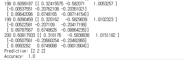
학습에서 사용되지 않았던 test set으로 계산했기 때문에 의미있는 정확도를 도출할 수 있다.
[Learning rate 선정에 따른 문제점]
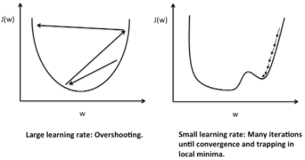
Large learning rate: Overshooting
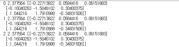
위와 동일한 코드에서 larning_rate = 1.5로 설정한 결과
[출력]
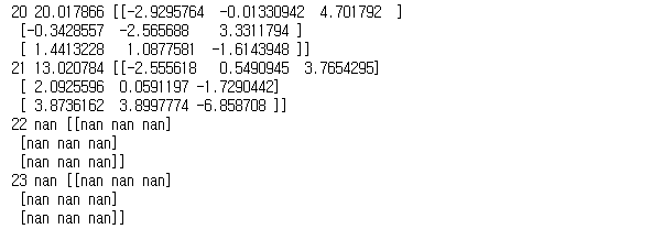
cost 값이 발산하고 학습이 안된다.
Small learning rate
위와 동일한 코드에서 learning_rate = 1e-20으로 설정한 결과
[출력]

step이 진행되어도 cost값의 변화가 거의 없다.
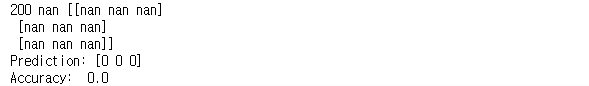
[데이터가 normalized 되어있지 않은 경우]
데이터의 값이 크거나 값이 들쑥날쑥한 경우, learning rate이 제대로 설정되어도 NaN을 만날 수 있다!
Non-normalized data로 linear regression 모델을 구현
import tensorflow.compat.v1 as tf
import numpy as np
tf.disable_v2_behavior()
tf.set_random_seed(777)  # for reproducibility

xy = np.array([[828.659973, 833.450012, 908100, 828.349976, 831.659973],
              [823.02002, 828.070007, 1828100, 821.655029, 828.070007],
              [819.929993, 824.400024, 1438100, 818.97998, 824.159973],
              [816, 820.958984, 1008100, 815.48999, 819.23999],
              [819.359985, 823, 1188100, 818.469971, 818.97998],
              [819, 823, 1198100, 816, 820.450012],
              [811.700012, 815.25, 1098100, 809.780029, 813.669983],
              [809.51001, 816.659973, 1398100, 804.539978, 809.559998]])

x_data = xy[:, 0:-1]
y_data = xy[:, [-1]]

# placeholders for a tensor that will be always fed
X = tf.placeholder(tf.float32, [None, 4])
Y = tf.placeholder(tf.float32, [None, 1])
W = tf.Variable(tf.random_normal([4, 1]), name = 'weight')
b = tf.Variable(tf.random_normal([1]), name = 'bias')

hypothesis = tf.nn.softmax(tf.matmul(X, W) + b)
cost = tf.reduce_mean(tf.reduce_mean(tf.square(hypothesis - Y)))

# Minimize
optimizer = tf.train.GradientDescentOptimizer(learning_rate = 1e-5)
train = optimizer.minimize(cost)

sess = tf.Session()
sess.run(tf.global_variables_initializer())

for step in range(2001):
    cost_val, hy_val, _ = sess.run([cost, hypothesis, train], feed_dict = {X: x_data, Y: y_data})
    print(step, "Cost: ", cost_val, "\nPrediction:\n", hy_val)
Nan이 출력된다.
data를 normalize하여 문제를 해결한다.
MinMaxScalar()를 통해 데이터를 0과 1 사이의 값으로 normalize하면 값이 치우치지 않는다.
xy = MinMaxScalar(xy)'AI > 모두를 위한 ML (SungKim)' 카테고리의 다른 글
| [ML lab 08] Tensor Manipulation (0) | 2021.02.20 |
|---|---|
| [ML alb 07-2] Meet MNIST Dataset (0) | 2021.02.20 |
| [ML lab 06-2] TensorFlow로 Fancy Softmax Classification 구현하기 (0) | 2021.02.20 |
| [ML lab 06-1] TensorFlow로 Softmax Classification 구현하기 (0) | 2021.02.18 |
| [ML lab 05] TensorFlow로 Logistic Classification 구현하기 (0) | 2021.02.17 |
'AI/모두를 위한 ML (SungKim)' Related Articles
more

Comments