| 일 | 월 | 화 | 수 | 목 | 금 | 토 |
|---|---|---|---|---|---|---|
| 1 | 2 | 3 | ||||
| 4 | 5 | 6 | 7 | 8 | 9 | 10 |
| 11 | 12 | 13 | 14 | 15 | 16 | 17 |
| 18 | 19 | 20 | 21 | 22 | 23 | 24 |
| 25 | 26 | 27 | 28 | 29 | 30 | 31 |
Tags
- 모두를 위한 머신러닝
- join
- 백준
- Machine learning
- c++
- DFS
- Programmers
- 큐
- Neural Network
- 프로그래머스
- softmax
- 정렬
- mysql
- stl
- sung kim
- BOJ
- TensorFlow
- 모두를 위한 딥러닝
- SQL
- Queue
- 알고리즘 고득점 kit
- sort
- PIR
- CSAP
- ML
- Linear Regression
- 한화오션
- 시간초과
- deque
- deep learning
Archives
- Today
- Total
hello, world!
[ML lab 06-2] TensorFlow로 Fancy Softmax Classification 구현하기 본문
AI/모두를 위한 ML (SungKim)
[ML lab 06-2] TensorFlow로 Fancy Softmax Classification 구현하기
ferozsun 2021. 2. 20. 14:54[cross entropy cost를 더 간단하게 구하는 방법]

softmax_cross_entropy_with_logits() # 파라미터로 logits과 Y lable을 넘겨준다.
[Y의 모양을 0~N의 label에서 one hot 형태로 바꾸는 방법]
one_hot()
파라미터로 0부터 시작되는 Y, class의 개수를 넘겨준다.
input의 rank가 N이라면 output의 rank는 N+1이 된다. (차원이 커지며 아직 원하는 shape이 반환되지 않음!)
reshape()
위 one_hot()과 원하는 shape을 파라미터로 보낸다. (원하는 shape이 반환 됨!)
동물 정보(x_data)에 대한 어떤 동물인지 결과(y_data)를 학습시켜 예측하는 모델이다.
x_data: n개의 인스턴스가 17개의 측정값으로 구성된다. (hair, feathers, eggs, ..., fins, legs, tail 등 정보)
y_data: n개의 인스턴스가 1개의 결과치(label)로 구성된다. (0~6번 동물 label)
# data-04-zoo.cvs
1,0,0,1,0,0,1,1,1,1,0,0,4,0,0,1,0
1,0,0,1,0,0,0,1,1,1,0,0,4,1,0,1,0
0,0,1,0,0,1,1,1,1,0,0,1,0,1,0,0,3
1,0,0,1,0,0,1,1,1,1,0,0,4,0,0,1,0
. . .
1,0,1,0,1,0,0,0,0,1,1,0,6,0,0,0,5
1,0,0,1,0,0,1,1,1,1,0,0,4,1,0,1,0
0,0,1,0,0,0,0,0,0,1,0,0,0,0,0,0,6
0,1,1,0,1,0,0,0,1,1,0,0,2,1,0,0,1
import tensorflow.compat.v1 as tf
import numpy as np
tf.disable_v2_behavior()
xy = np.loadtxt('data-04-zoo.cvs', delimiter = ',', dtype = np.float32)
x_data = xy[:, 0:-1]
y_data = xy[:, [-1]]
nb_classes = 7 # 0 ~ 6
X = tf.placeholder(tf.float32, [None, 16])
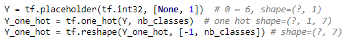
Y = tf.placeholder(tf.int32, [None, 1]) # 0~ 6
# Y는 그냥 0부터 6까지의 숫자이기 때문에 one hot으로 바꿔줘야한다.
Y_one_hot = tf.one_hot(Y, nb_classes) # one hot (차원이 1 늘어남)
Y_one_hot = tf.reshape(Y_one_hot, [-1, nb_classes]) # 원하는 shape으로 바꿈
W = tf.Variable(tf.random_normal([16, nb_classes]), name = 'weight')
b = tf.Variable(tf.random_normal([nb_classes]), name = 'bias')
# tf.nn.softmax computes softmax activations
# softmax = exp(logits) / reduce_sum(exp(logits), dim)
logits = tf.matmul(X, W) + b
hypothesis = tf.nn.softmax(logits)
# Cross entropy cost/loss
cost_i = tf.nn.softmax_cross_entropy_with_logits(logits = logits, labels = Y_one_hot)
cost = tf.reduce_mean(cost_i)
optimizer = tf.train.GradientDescentOptimizer(learning_rate = 0.1).minimize(cost)
# 학습
cost = tf.reduce_mean(cost_i)
optimizer = tf.train.GradientDescentOptimizer(learning_rate = 0.1).minimize(cost)
prediction = tf.argmax(hypothesis, 1)
correct_prediction = tf.equal(prediction, tf.argmax(Y_one_hot, 1))
accuracy = tf.reduce_mean(tf.cast(correct_prediction, tf.float32)) # 예측과 일치한 것의 평균을 낸 정확도
# Launch graph
with tf.Session() as sess:
sess.run(tf.global_variables_initializer())
for step in range(2000):
sess.run(optimizer, feed_dict = {X: x_data, Y: y_data})
if step % 100 == 0:
loss, acc = sess.run([cost, accuracy], feed_dict = {X: x_data, Y: y_data})
print("Step: {:5}\tLoss: {:.3f}\tAcc: {:.2%}".format(step, loss, acc))
# Let's see if we can predict
pred = sess.run(prediction, feed_dict = {X: x_data})
# y_data: (N,1) = flatten => (N, ) matches pred.shape
for p, y in zip(pred, y_data.flatten()):
print("[{}] Prediction: {} True Y: {}".format(p == int(y), p, int(y)))[출력]
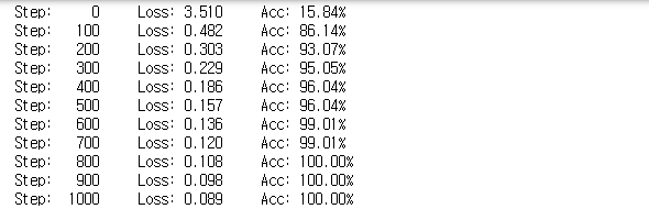

정확도가 100%까지 학습된다. 예측값과 실제 Y값이 일치한다.
'AI > 모두를 위한 ML (SungKim)' 카테고리의 다른 글
| [ML alb 07-2] Meet MNIST Dataset (0) | 2021.02.20 |
|---|---|
| [ML lab 07-1] training/test dataset, learning rate, normalization (0) | 2021.02.20 |
| [ML lab 06-1] TensorFlow로 Softmax Classification 구현하기 (0) | 2021.02.18 |
| [ML lab 05] TensorFlow로 Logistic Classification 구현하기 (0) | 2021.02.17 |
| [ML lab 04-2] TensorFlow로 파일에서 데이타 읽어오기 (0) | 2021.02.17 |
'AI/모두를 위한 ML (SungKim)' Related Articles
more

Comments