
| 일 | 월 | 화 | 수 | 목 | 금 | 토 |
|---|---|---|---|---|---|---|
| 1 | 2 | 3 | ||||
| 4 | 5 | 6 | 7 | 8 | 9 | 10 |
| 11 | 12 | 13 | 14 | 15 | 16 | 17 |
| 18 | 19 | 20 | 21 | 22 | 23 | 24 |
| 25 | 26 | 27 | 28 | 29 | 30 | 31 |
- c++
- 프로그래머스
- TensorFlow
- Machine learning
- 백준
- deque
- Linear Regression
- SQL
- DFS
- Queue
- CSAP
- ML
- 큐
- PIR
- mysql
- sort
- deep learning
- 시간초과
- join
- 알고리즘 고득점 kit
- 한화오션
- Neural Network
- stl
- 정렬
- 모두를 위한 머신러닝
- 모두를 위한 딥러닝
- sung kim
- BOJ
- softmax
- Programmers
- Today
- Total
목록TensorFlow (8)
hello, world!
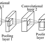 [ML lab 11-2] MNIST 99% with CNN
[Simple CNN] import numpy as np import tensorflow as tf import random mnist = tf.keras.datasets.mnist (x_train, y_train), (x_test, y_test) = mnist.load_data() x_test = x_test / 255 x_train = x_train / 255 x_train = x_train.reshape(x_train.shape[0], 28, 28, 1) x_test = x_test.reshape(x_test.shape[0], 28, 28, 1) # one hot encode y data y_train = tf.keras.utils.to_categorical(y_train, 10) y_test = ..
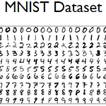 [ML alb 07-2] Meet MNIST Dataset
import tensorflow as tf learning_rate = 0.001 batch_size = 100 training_epochs = 15 nb_classes = 10 # download mnist dataset mnist = tf.keras.datasets.mnist (x_train, y_train), (x_test, y_test) = mnist.load_data() # normalizing data x_train, x_test = x_train / 255.0, x_test / 255.0 # change data shape print(x_train.shape) # (60000, 28, 28) x_train = x_train.reshape(x_train.shape[0], x_train.shap..
Logistic Classification은 정확도가 높은 알고리즘이다. Binary classification: 둘 중 하나를 골라 결과를 내는 것 (machine: 0 또는 1) 공부 시간(x_data)에 대한 P/F 결과(fail:0 / pass:1)(y_data)를 학습시킨 모델이다. x_data: n개의 인스턴스가 2개의 측정값으로 구성된다. y_data: n개의 인스턴스가 1개의 결과치로 구성된다. import tensorflow.compat.v1 as tf tf.disable_v2_behavior() x_data = [[1, 2], [2, 3], [3, 1], [4, 3], [5, 3], [6, 2]] y_data = [[0], [0], [0], [1], [1], [1]] # placehol..
[Slicing examples] b = np.array([[1, 2, 3, 4], [5, 6, 7, 8], [9, 10, 11, 12]]) # array([[1, 2, 3, 4], # [5, 6, 7, 8], # [9, 10, 11, 12]]) b[:, 1] # array([ 2, 6, 10]) b[-1] # array([ 9, 10, 11, 12]) b[-1, :] # array([ 9, 10, 11, 12]) b[-1, ...] # array([ 9, 10, 11, 12]) b[0:2, :] # array([[1, 2, 3, 4], # [5, 6, 7, 8]]) [Loading data from file] x_data와 y_data가 많아짐에 따라 소스코드에 전부 적는 것이 무리가 있다. 따라서 텍..
[multi-variable] import tensorflow.compat.v1 as tf tf.disable_v2_behavior() x1_data = [73., 93., 89., 96., 73.] x2_data = [80., 88., 91., 98., 66.] x3_data = [75., 93., 90., 100., 70.] y_data = [152., 185., 180., 196., 142.] # placeholders for a tensor that will be always fed. x1 = tf.placeholder(tf.float32) x2 = tf.placeholder(tf.float32) x3 = tf.placeholder(tf.float32) Y = tf.placeholder(tf.fl..
cost 함수를 그려서 최저점을 확인한다. import tensorflow.compat.v1 as tf import matplotlib.pyplot as plt tf.disable_v2_behavior() X = [1, 2, 3] Y = [1, 2, 3] W = tf.placeholder(tf.float32) # Our hypothesis for linear model X * W hypothesis = X * W # cost/loss function cost = tf.reduce_mean(tf.square(hypothesis - Y)) # Launch the graph in a session sess = tf.Session() # Initializes global variables in the graph..
X가 1일 때 Y가 1, X가 2일 때 Y가 2, X가 3일 때 Y가 3인 값들을 보고 학습한 후 cost function이 최소가 되는 hypothesis의 W(weight)와 b(bias)예측해 보라는 예제이다. import tensorflow.compat.v1 as tf tf.disable_v2_behavior() ## 그래프 구현 # X and Y data x_train = [1, 2, 3] y_train = [1, 2, 3] W = tf.Variable(tf.random_normal([1]), name = 'weight') b = tf.Variable(tf.random_normal([1]), name = 'bias') # hypothesis = XW + b hypothesis = x_train ..
TensorFlow 설치 후 Jupyter Notebook을 이용한다. 본 version은 2.3.0이지만 version 1.xx를 사용하기 위해 v1을 import한다. constant 노드를 생성한 후 세션을 만들어 실행(run())한다. 각 노드가 어떤 tensor인지 정보만 출력된다. session을 만든 후 run을 통해서 graph의 노드를 실행하면 원하는 결과값이 출력된다. placeholder 노드를 사용하면 값을 미리 정해두지 않고, 프로그램이 돌아가는 시점에 정할 수 있다. 변수의 type만 정해 두고, feed_dict를 통해 parameter로 값을 넘겨 받아 graph를 실행시킨다. (array를 통해 n개의 값을 넘겨줄 수 있다.) ranks: 몇 차원 array인가? shape..